Due 7/24 at 5:30pm.
Implement the classic Dijkstra’s shortest path algorithm and optimize it for maps. Such algorithms are widely used in geographic information systems (GIS) including MapQuest and GPS-based car navigation systems.
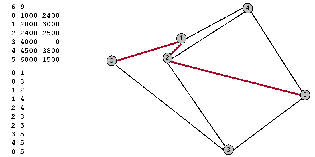
Maps. For this assignment we will be working with maps, or graphs whose vertices are points in the plane and are connected by edges whose weights are Euclidean distances. Think of the vertices as cities and the edges as roads connected to them. To represent a map in a file, we list the number of vertices and edges, then list the vertices (index followed by its x and y coordinates), then list the edges (pairs of vertices), and finally the source and sink vertices. For example, input6.txt represents the map below:
Dijkstra’s algorithm. Dijkstra’s algorithm is a classic solution to the shortest path problem on a weighted graph. The basic idea is not difficult to understand. We maintain, for every vertex in the graph, the length of the shortest known path from the source to that vertex, and we maintain these lengths in a priority queue. Initially, we put all the vertices on the queue with an artificially high priority and then assign priority 0.0 to the source. The algorithm proceeds by taking the lowest-priority vertex off the PQ, then checking all the vertices that can be reached from that vertex by one edge to see whether that edge gives a shorter path to the vertex from the source than the shortest previously-known path. If so, it lowers the priority to reflect this new information.
Here is a step-by-step description that shows how Dijkstra’s algorithm finds the shortest path 0-1-2-5 from 0 to 5 in the example above:
process 0 (0.0)
    lower 3 to 3841.9
    lower 1 to 1897.4
process 1 (1897.4)
    lower 4 to 3776.2
    lower 2 to 2537.7
process 2 (2537.7)
    lower 5 to 6274.0
process 4 (3776.2)
process 3 (3841.9)
process 5 (6274.0)
This method computes the length of the shortest path. To keep track of the path, we also maintain for each vertex, its predecessor on the shortest path from the source to that vertex. The files EuclideanGraph.java, Point.java, IndexPQ.java, IntIterator.java, and Dijkstra.java provide a bare bones implementation of Dijkstra’s algorithm for maps, and you should use this as a starting point. The client program ShortestPath.java solves a single shortest path problem and plots the results using turtle graphics. The client program Paths.java solves many shortest path problems and prints the shortest paths to standard output. The client program Distances.java solves many shortest path problems and prints only the distances to standard output.
Your goal. Optimize Dijkstra’s algorithm so that it can process thousands of shortest path queries for a given map. Once you read in (and optionally preprocess) the map, your program should solve shortest path problems in sublinear time. One method would be to precompute the shortest path for all pairs of vertices; however you cannot afford the quadratic space required to store all of this information. Your goal is to reduce the amount of work involved per shortest path computation, without using excessive space. We suggest a number of potential ideas below which you may choose to implement. Or you can develop and implement your own ideas.
- Idea 1. The naive implementation of Dijkstra’s algorithm examines all V vertices in the graph. An obvious strategy to reduce the number of vertices examined is to stop the search as soon as you discover the shortest path to the destination. With this approach, you can make the running time per shortest path query proportional to E’ log V’ where E’ and V’ are the number of edges and vertices examined by Dijkstra’s algorithm. However, this requires some care because just re-initializing all of the distances to ∞ would take time proportional to V. Since you are doing repeated queries, you can speed things up dramatically by only re-initializing those values that changed in the previous query.
- Idea 2. You can cut down on the search time further by exploiting the Euclidean geometry of the problem, as described in Sedgewick 21.5. For general graphs, Dijkstra’s relaxes edge v-w by updating wt[w] to the sum of wt[v] plus the distance from v to w. For maps, we instead update wt[w] to be the sum of wt[v] plus the distance from v to w plus the Euclidean distance from w to d minus the Euclidean distance from v to d. This is known as the A* algorithm. This heuristics affects performance, but not correctness. (See Sedgewick 21.5 for a proof of correctness.)
- Idea 3. Use a faster priority queue. There is some room for optimization in the supplied priority queue. You could also consider using a multiway heap.
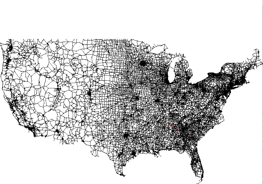
Testing. The file usa.txt contains 87,575 intersections and 121,961 roads in the continental United States. The graph is very sparse – the average degree is 2.8. Your main goal should be to answer shortest path queries quickly for pairs of vertices on this network. Your algorithm will likely perform differently depending on whether the two vertices are nearby or far apart. We provide input files that test both cases. You may assume that all of the x and y coordinates are integers between 0 and 10,000.
Deliverables. Improve the bare bones implementation by using some of the ideas described above together with your ingenuity. You may modify Dijkstra.java, EuclideanGraph.java, Point.java, and IndexPQ.java. However, your code should work with any of our three client programs. Submit all of the files needed to compile your program, except Turtle.java, StdIn.java, and In.java. Also, submit a memo.txt file using the one provided as a template. Describe and justify your approach. Compare your approach to the bare bones implementation. In particular give the average number of vertices examined.
View the source needed for this assignment here: https://github.com/ieee8023/cs210-summer2014
You can test your code using the files usa-10.txt and usa-1000long.txt on the map usa.txt
## usa-10.txt contains queries to as the dijkstra.distance(s, d) method
$ cat usa-10.txt
      0   87428
   1000   50000
   2000    2200
   2200    2000
   6000    3000
  50000   51000
  65000   22000
  12345   54321
   9999    9999
  62860   62809
Now we can run these queries on the map using the Distances class. It will print out the distances for each query. You will need to make sure that the distances are the same with and without your modification.
$ java Distances usa.txt  < usa-10.txt
Done reading the graph usa.txt
Enter query pairs from stdin
4398.266983154727
2937.891782062475
48.721349351738354
48.72134935173836
5768.470098906614
665.9934083546462
2182.392176416482
5485.618212015974
0.0
3.414213562373095
We can time the difference using the “time” command line tool. You can also avoid printing the path distances by adding “> /dev/null” to prevent stdout from showing. The times will still print.
$ time java Distances usa.txt   /dev/null
Done reading the graph usa.txt
Enter query pairs from stdin

real	0m0.887s
user	0m1.396s
sys	0m0.078s

$ time java Distances usa.txt   /dev/null
Done reading the graph usa.txt
Enter query pairs from stdin

real	0m33.920s
user	0m34.321s
sys	0m0.231s
Grading (total 25 points):
5 points: Decrease running time
10 points: Decrease running time and path distance is the same as before
8 points: Explain in your memo.txt what you did and why it decreased running time. Note what files you modified and explain your changes. Showing code fragments that you changed is best.
2 points: Easy to grade, compiles on users
This assignment was developed by Bob Sedgewick and Kevin Wayne. Copyright © 2004.