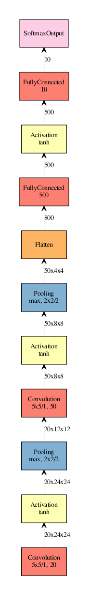
Convolutional Neural Networks can be visualized as computation graphs with input nodes where the computation starts and output nodes where the result can be read. Here the models that are provided with mxnet are compared using the mx.viz.plot_network method. The output node is at the top and the input node is at the bottom.
import find_mxnet
import mxnet as mx
import importlib

name = "inception-v3"
net = importlib.import_module("symbol_" + name).get_symbol(2)
a = mx.viz.plot_network(net, shape={"data":(1, 1, 299, 299)}, node_attrs={"shape":'rect',"fixedsize":'false'})
a.render(name)
| LeNet 28×28 (1998) |
AlexNet 224×224 (2012) |
VGG 224×224 (9/2014) |
GoogLeNet 224×224 (9/2014) |
Inception BN 224×224 (2/2015) |
Inception V3 299×299 (12/2015) |
Resnet (n=9, 56 Layers) 28×28 (12/2015) |
 |
 |
 |
 |
 |
 |
 |